At MakinaRocks, we specialize in anomaly detection, amongst other things. But what exactly is anomaly detection? In this post, we will explore a few standard methods used to conduct anomaly detection and introduce our approach.

Anomaly Detection, also known as fraud or novelty detection, is the classification of normal and anomalous data. Anomaly Detection is essential in situations such as credit card fraud detection, video surveillance, autonomous driving, and industrial machinery maintenance.

Binary Classification

As the name suggests, binary classification models predict the classification of two different classes. For instance, binary classification can be deployed to determine if something is spam or not spam, correct or incorrect, or any two binary classes. To this end, it is widely used to perform anomaly detection.

The image below depicts classification, in which there is a boundary separating normal and abnormal data, and anomaly detection, in which anomalous data refers to data distributed outside of the normal data range.

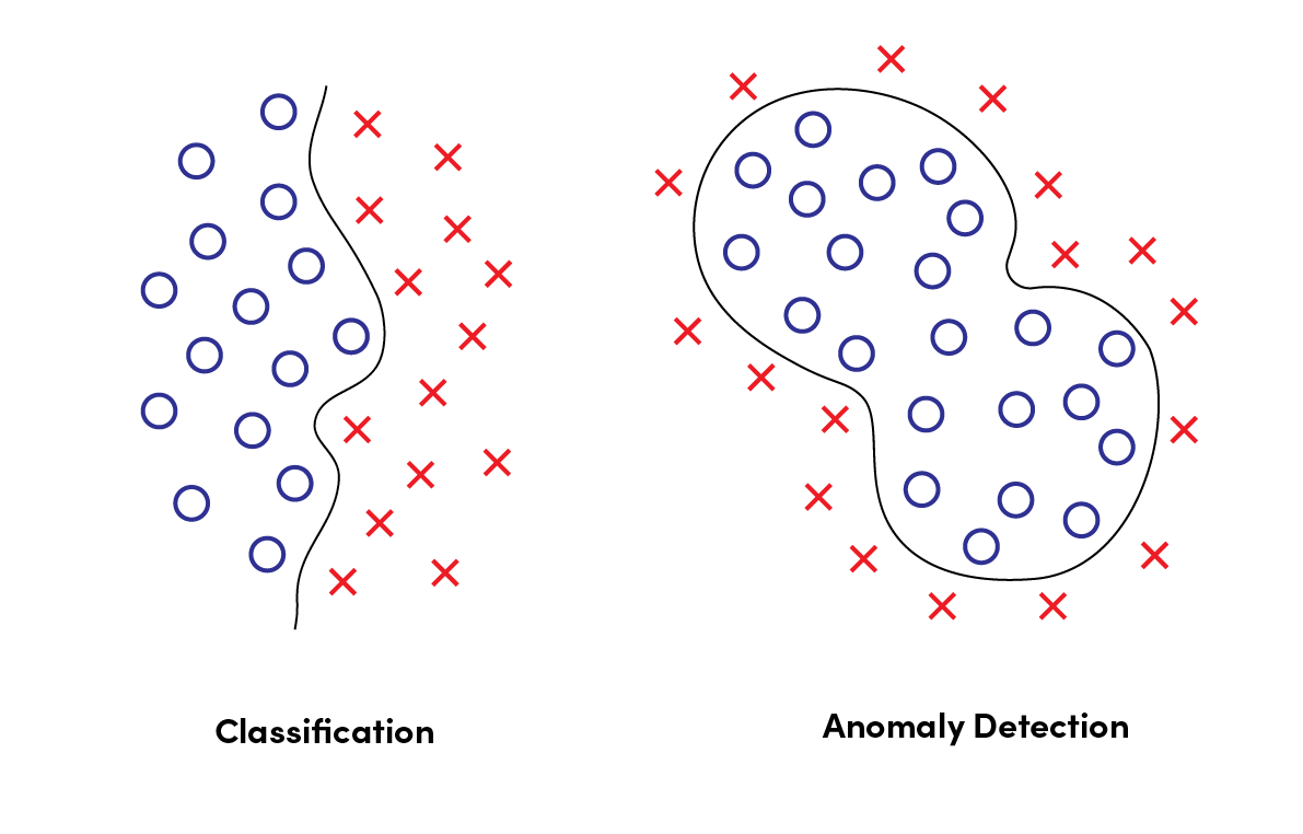
However, in the highly dynamic conditions of the real world, anomalies are not merely binary. Anomalous activity typically occurs sporadically, in abnormal patterns. Even if we were to define an anomalous class by training the model with anomalous patterns, we would still not be able to narrow down and learn all of the patterns of the anomalous data.

Principal Component Analysis (PCA)

Another common method of anomaly detection is Principal Component Analysis or PCA. A “special” form of autoencoder, PCA maps material from high-dimensional spaces to low-dimensional spaces with Singular Value Decomposition (SVD), as depicted below.

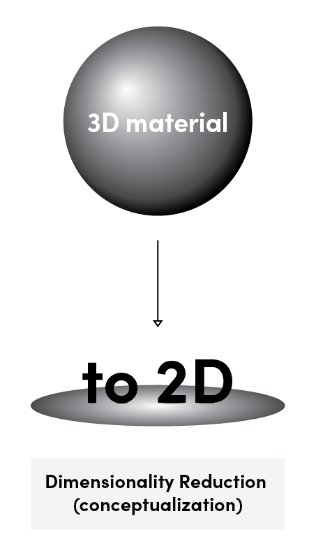
During PCA, features can be extracted and compared to determine if anomalous or not through linear dimensionality reduction. However, due to the limitations of dimensionality reduction, PCA is not always the most viable solution. In cases such as the one depicted below, anomalous samples cannot be detected.

Semi-supervised learning

Semi-supervised learning algorithms are trained from a mixed batch of labeled and unlabeled instances.

An effective method of improving accuracy, semi-supervised learning, is widely implemented to detect and classify anomalies. They can be classified into two different cases: unimodal and multimodal normality cases.

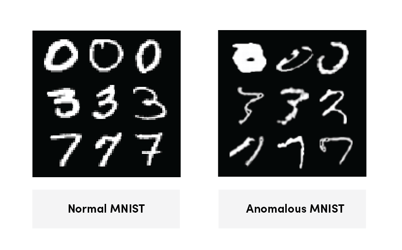
Unimodal normality cases, or one-class classification, refer to situations in which normality is represented by a single set of normal features. This is exemplified by the image below, in which we have a set of “normal” MNIST samples on the left and anomalous samples on the right.

With countless factors to consider, creating a model for the real world is a challenge, and normality in the real world cannot be defined by a single set of patterns. Given the dynamic conditions, real world problems are generally defined as multimodal normality cases.

We will take a car engine, for instance. If we were to perform anomaly detection on a car engine, the engine could be defined into four different states: intake, compression, explosion, and exhaust. As each state differs from one another, a more complex method is required to train and evaluate a model for this problem.

We can better explain the model training and evaluation process for said scenarios with MNIST. For instance, model training can be performed with nine classes. Once the training is complete, the remaining “1” class, or the anomaly, can be used to evaluate if the model accurately classified the cases.

Due to the complex nature of this method, training is difficult to conduct, and anomaly detection models have been known to show lower performance.

Autoencoders (AE)

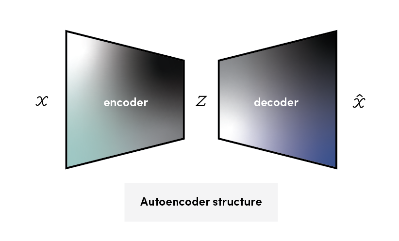
An autoencoder extracts features with dimensionality reduction--just not linearly. What an autoencoder does is to extract features by compressing and decompressing data. Let’s take an MP3 recording, for instance. When you listen to an MP3 recording, you’re actually listening to data compressed after discarding data in the frequency range not perceptible to the human ear.

In doing so, autoencoders teach themselves how to extract features through the process of encoding and decoding. However, due to the MSE loss function in which the autoencoder predicts the average value for uncertain areas, results are often unclear.

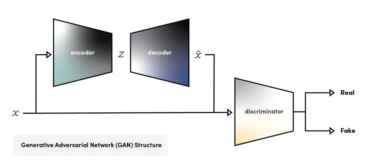
Generative Adversarial Network (GAN)

There are two components of the Generative Adversarial Network: the generative network and the discriminative network. The generative network learns to create “fake” examples while the discriminative network learns to distinguish said “fake” examples from real world examples. Since the model is trained through the hostile learning between the generator and the discriminator, it does not possess a module that performs dimensionality reduction.

To conduct anomaly testing, a module for dimensionality reduction is necessary. While existing GAN-based anomaly detection methods suggest various methods to solve this issue, the balanced learning of the generator and the discriminator and the shortcomings of MSE act as a significant obstacle.

References
[1] Ki Hyun Kim, Operational AI: Building a Lifelong Learning Anomaly Detection System, DEVIEW, 2019
[2] Jinwon An et al., Variational Autoencoder based Anomaly Detection using Reconstruction Probability, SNU Data Mining Center, 2015
[3] Anh Nguyen et al., Deep Neural Networks are Easily Fooled: High Confidence Predictions for Unrecognizable Images, CVPR, 2015
[4] Ian J. Goodfellow et al., Explaining and Harnessing Adversarial Examples, Arxiv, 2014
[5] Ki Hyun Kim et al., RaPP: Novelty Detection with Reconstruction along Projection Pathway, ICLR, 2020
[6] Stanislav Pidhorskyi et al., Generative Probabilistic Novelty Detection with Adversarial Autoencoders, NeurIPS, 2018
[7] Lukas Ruff et al., Deep One-Class Classification, ICML, 2018
[8] Siqi Wang et al., Effective End-to-end Unsupervised Outlier Detection via Inlier Priority of Discriminative Network, NeurIPS, 2019
[9] Thomas Schlegl et al., Unsupervised Anomaly Detection with Generative Adversarial Networks to Guide Marker Discovery, Arxiv, 2017
[10] Houssam Zenati et al., Efficient GAN-Based Anomaly Detection, Arxiv, 2018
[11] Ilyass Haloui et al., Anomaly detection with Wasserstein GAN, 2018
[12] Izhak Golan et al., Deep Anomaly Detection Using Geometric Transformations, NeurIPS, 2018

You can’t talk about the industrial sector without talking about industrial machinery. Neither can we. At MakinaRocks, we aim to make industrial technology intelligent and deliver it as transformative solutions.

We believe in tailoring our AI solutions to meet the needs of our clients, which not only includes increased technical specifications involving efficiency and performance metrics, but something just as important: convenience.

There are a number of ways to maintain industrial machinery. If you search around, you will most likely come across these terms: preventive maintenance and predictive maintenance.

While both refer to preventing industrial machinery breakdown (and factory shutdowns – yikes!), preventive maintenance generally involves scheduling an expert to come down to your factory once every few months to take a look at your machinery and see if anything needs fixing. On the other hand, predictive maintenance refers to using data to predict when the machine will break down, so you can call in an expert prior to the anticipated breakdown. MakinaRocks solutions take the concept of predictive maintenance a few steps further.

What we’ve built is a predictive maintenance solution based on AI—excelling in accuracy and performance.

In this post, we will explain our novel anomaly detection metric behind our state-of-the-art anomaly detection solution: Reconstruction along Projection Pathway (RaPP), a concept acknowledged by the International Conference on Learning Representations (ICLR) in 2020.

What is RaPP?

RaPP is our proposed anomaly detection metric for autoencoders—drastically improving the anomaly detection performance without changing anything about the training process.

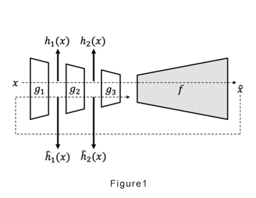
RaPP redefines the anomaly detection metric by enhancing the reconstruction process. Reconstruction is the difference between the input and output of an autoencoder. RaPP extends this concept to what we refer to as the hidden layers in our paper. This is done by feeding the initial output to the (very same) autoencoder again and aggregating the intermediate activation vectors from the hidden layers.

SAP & NAP

To reiterate, RaPP enables the comparison of the output values produced in the encoder and decoder’s hidden spaces. We implemented two different methods to measure performance: RaPP’s Simple Aggregation along Pathway (SAP), and RaPP’s Normalized Aggregation along Pathway (NAP).

Figure 2 exemplifies SAP, but when the distribution is so, it merely depicts the distance from the origin. A more suitable approach would be to calculate the distribution as exemplified in figure 3, which is equivalent to achieving the Mahalnobis distance. To do this, we can attain a normalized distance by applying Singular Value Decomposition (SVD) to the hidden reconstruction error of each layer from the training set. This concept is also known as RAPP’s NAP.

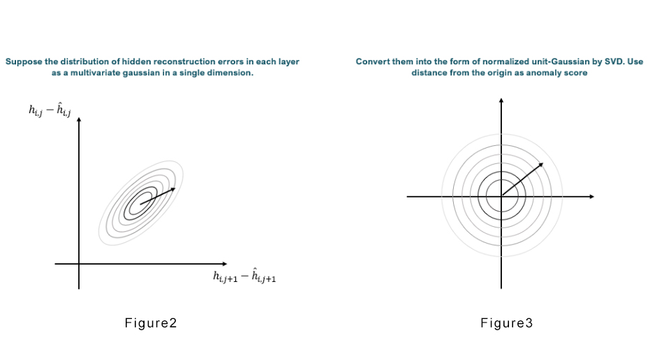
With SAP and NAP, a more accurate anomaly detection process may be performed by producing an anomaly score with the scalar value from the difference between multiple layers. Please refer to our paper for a more in-depth look at our methodology.

Our RaPP results

We performed numerous experiments to verify the effectiveness of RaPP. We began by using widely known and accepted datasets such as MNIST and FMNIST to compare the performance of our model with research from published, peer edited papers. The results are as follows:

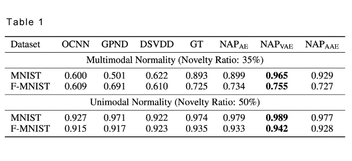
As you can see from the results, when NAP is applied to different autoencoders, we found that our results were far superior to the results in published papers. Namely, when NAP was applied to Variational Autoencoder (VAE), we were able to see the most significant results.

Further, we were able to prove the effectiveness of RaPP in multimodal normality cases as shown in the results below.

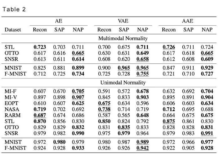
Upon implementation of RaPP, all but STL (steel) showed improvement in performance in multimodal normality cases. RaPP also proved to be more effective in 6 out of 10 instances in unimodal normality cases.

MakinaRocks’s transformative solution for predictive maintenance: ADS

Our RaPP anomaly score metric is featured in our Anomaly Detection Suite (ADS), empowering the solution to predict machinery breakdown with increased accuracy.

For more information about ADS, contact us at contact@makinarocks.ai
Want to know what we do? Visit us at www.makinarocks.ai
To read our ICLR 2020 accredited RaPP paper: https://iclr.cc/virtual_2020/poster_HkgeGeBYDB.html

References 

[1] Ki Hyun Kim et al., RaPP: Novelty Detection with Reconstruction along Projection Pathway, ICLR, 2020 
[2] Lei et al., Geometric Understanding of Deep Learning, Arxiv, 2018 
[3] Stanislav Pidhorskyi et al., Generative Probabilistic Novelty Detection with Adversarial Autoencoders, NeurIPS, 2018 
[4] Kingma et al., Auto-Encoding Variational Bayes, ICLR, 2014 
[5] Makhzani et al., Adversarial autoencoders. Arxiv, 2015. 
[6] Raghavendra Chalapathy et al., Anomaly detection using one-class neural networks. arXiv preprint arXiv:1802.06360, 2018. 
[7] Lukas Ruff et al., Deep one-class classification. In ICML, 2018. 
[8] Izhak Golan and Ran El-Yaniv. Deep anomaly detection using geometric transformations. NIPS, 2018. 
[9] Ki Hyun Kim, Operational AI: Building a Lifelong Learning Anomaly Detection System, DEVIEW, 2019